Reproducible Urban Heat Island Modeling for Bengaluru

Abstract

The present research proposes a workflow for Urban Heat Island analysis for Bengaluru, utilizing multiple years of Earth Observation and interpretable machine learning. The methodology emphasizes spatial leakage control, multiple validation levels, and fixed artifacts.

The approach stacks Sentinel-2 and Landsat imagery for 2020-2025, applies physics-informed feature verification, and trains an XGBoost regressor with spatial block cross-validation. Held-out validation achieves an RMSE of 3.31 K and an R2 of 0.554. Regional validation estimates urban and rural mean temperatures of 310.8 K and 308.8 K, yielding a UHI intensity of 1.97 K.

Samples 10.2M aligned pixel samples

Tiles 164 spatially aligned tiles

Hold-out RMSE 3.31 K Level-1 pixel hold-out

Hold-out R2 0.554 explained variance

UHI intensity 1.97 K urban minus rural

Problem Statement and Gap

Most Earth Observation based UHI analyses demonstrate predictive capability, but they often under-specify the controls used for spatial leakage, traceability of execution, and reproducibility. In geospatial regression, adjacent pixels and nearby tiles are autocorrelated; random splits can therefore overstate generalization.

Bengaluru adds two practical complications: strong seasonality and heterogeneous land cover. Vegetation, water, built-up surfaces, and temporal drift all affect land surface temperature, so the validation procedure needs to be spatially aware and physically interpretable.

The contribution is not a new backbone architecture, but a reproducible and leakage-aware evaluation framework for EO-based UHI regression.

Methodology

The workflow links EO ingestion, seasonal alignment, spatial block validation, model training, regional validation, and checksum-based artifact locking into one execution protocol.

Fig. 1. Interactive methodology map. Hover or tap a stage to inspect how the workflow moves from multi-year Earth Observation stacks to leakage-aware validation and locked artifacts.

Selected stage

EO ingestion

Multi-year Sentinel-2 and Landsat imagery are stacked into aligned Earth Observation inputs before seasonal aggregation and feature checks.

2020-2025: time span
aligned rasters: artifact

Predicted land-surface temperature at year y, season s, and pixel p is modeled as:

T_pred(y,s,p) = f(x(y,s,p))

Here, x(y,s,p) is the feature vector for the corresponding year, season, and pixel. Features include NDVI, NDBI, latitude, longitude, seasonal variables, and WorldCover-derived class variables.

Validation Design

The experiment uses two validation levels. Level-1 compares model predictions against held-out Landsat-derived targets at the pixel level. Level-2 checks regional urban-rural thermal contrast and seasonal consistency against MODIS seasonal means.

ΔT_UHI = T_{urban mean} - T_{rural mean}

Table 1. Model and validation metrics.
Evaluation level	Metric	Value
Spatial CV	RMSE	3.487 K
Spatial CV	R2	0.527
Level-1 hold-out	RMSE	3.31 K
Level-1 hold-out	MAE	2.34 K
Level-1 hold-out	R2	0.554
Level-1 hold-out	Bias	+0.75 K
Level-1 hold-out	N	973,407 pixels
Level-2 regional	Urban mean LST	310.8 K
Level-2 regional	Rural mean LST	308.8 K
Level-2 regional	UHI intensity	1.97 K

Prediction and UHI Results

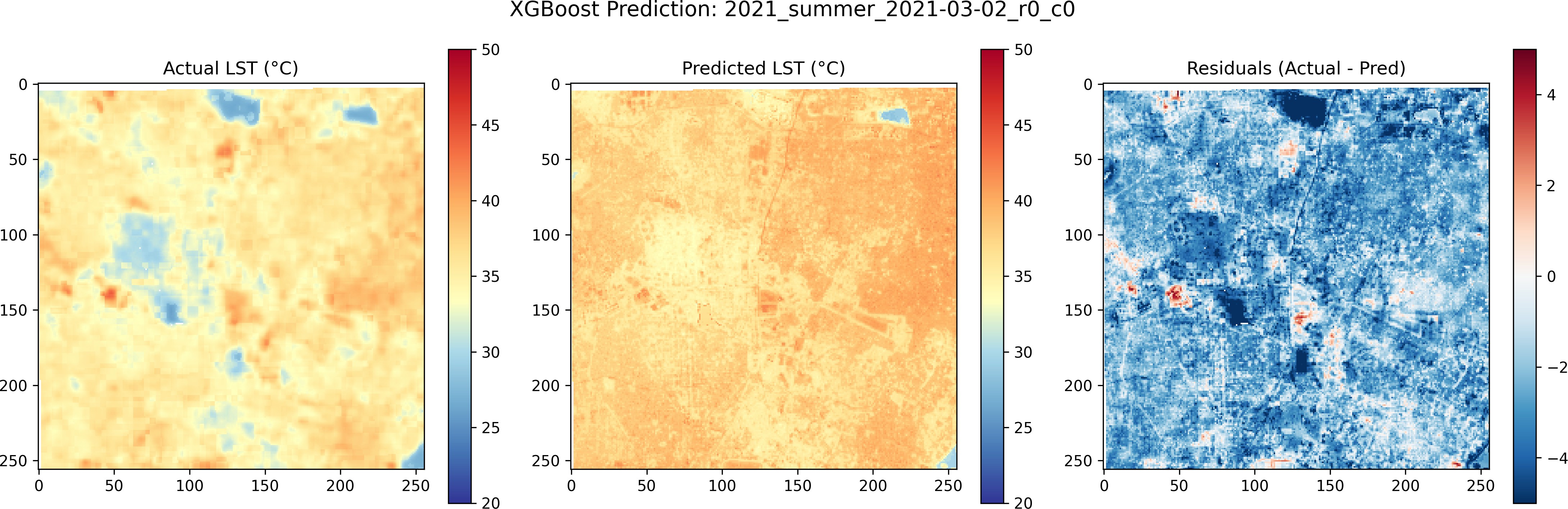
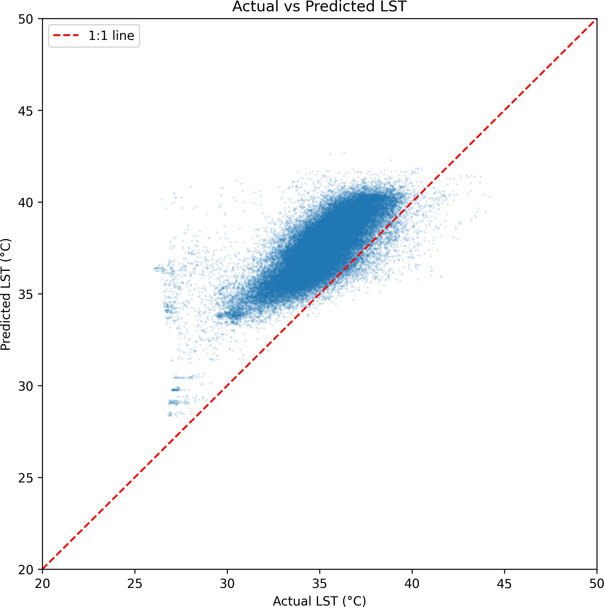
The prediction map shows spatial thermal structure across evaluation tiles. Warm and cool clusters provide a qualitative check of the expected urban-rural contrast, while the scatter plot summarizes pixel-level agreement between observed and predicted LST.

Actual LST, predicted LST, and residual map for an evaluation tile. — Fig. 2. Prediction map and residual structure for an evaluation tile. The panel preserves the original paper figure.

Scatter plot comparing actual and predicted land surface temperature. — Fig. 3. Observed versus predicted LST. The diagonal line represents perfect agreement; spread around the line shows residual error.

Table 2. Seasonal urban-rural UHI from the Step-12 drift run.
Year-season	Urban (K)	Rural (K)	UHI (K)
2020 Summer	312.8	310.9	1.95
2020 Winter	302.2	300.8	1.35
2021 Summer	310.9	309.6	1.37
2021 Winter	306.6	304.3	2.29
2022 Summer	310.4	308.8	1.54
2022 Winter	302.5	301.0	1.52
2023 Summer	312.2	310.3	1.85
2023 Winter	305.4	303.8	1.61
2024 Summer	312.3	311.0	1.31
2024 Winter	302.8	301.3	1.57
2025 Summer	311.9	310.0	1.87
2025 Winter	304.2	302.5	1.62

SHAP-Based Interpretability

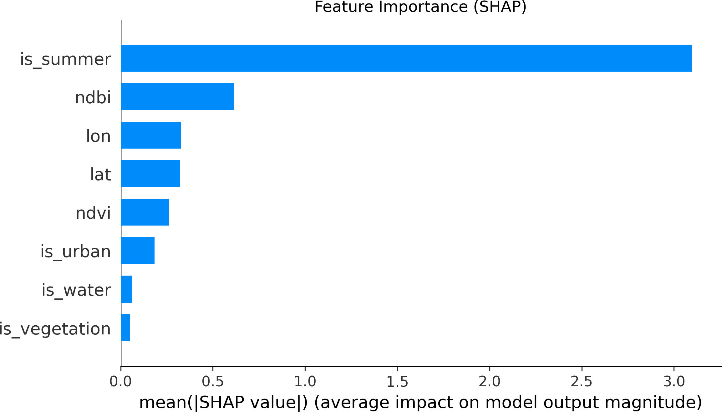
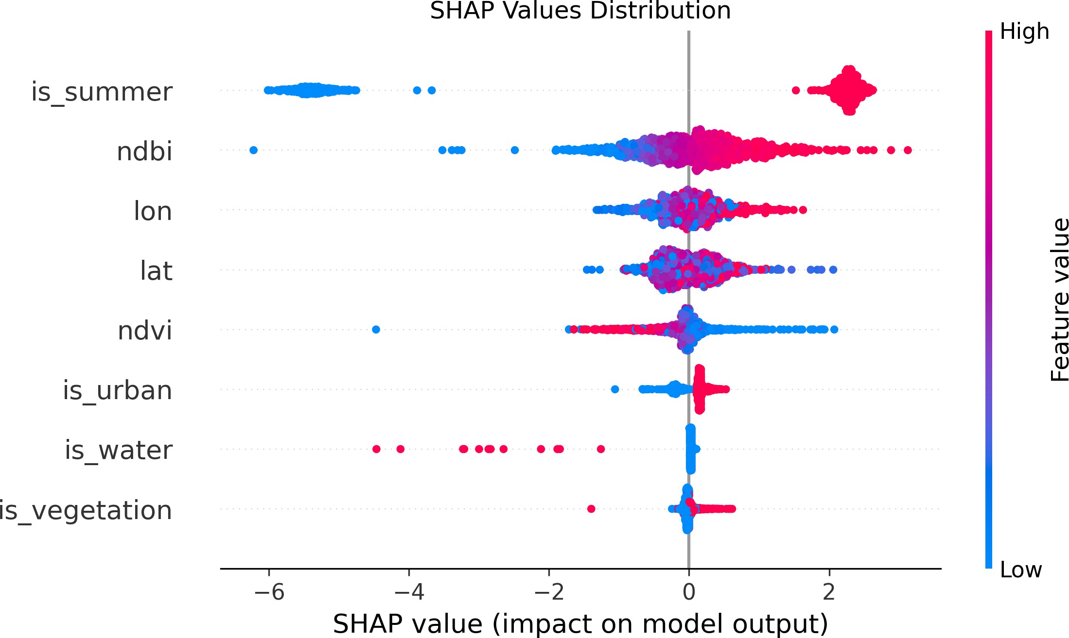
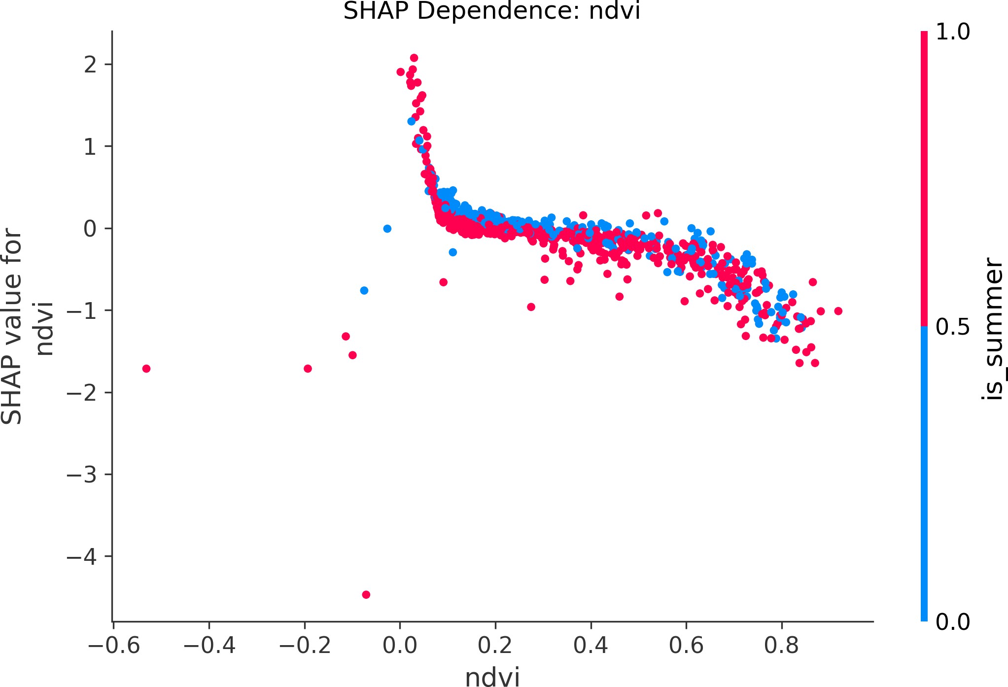
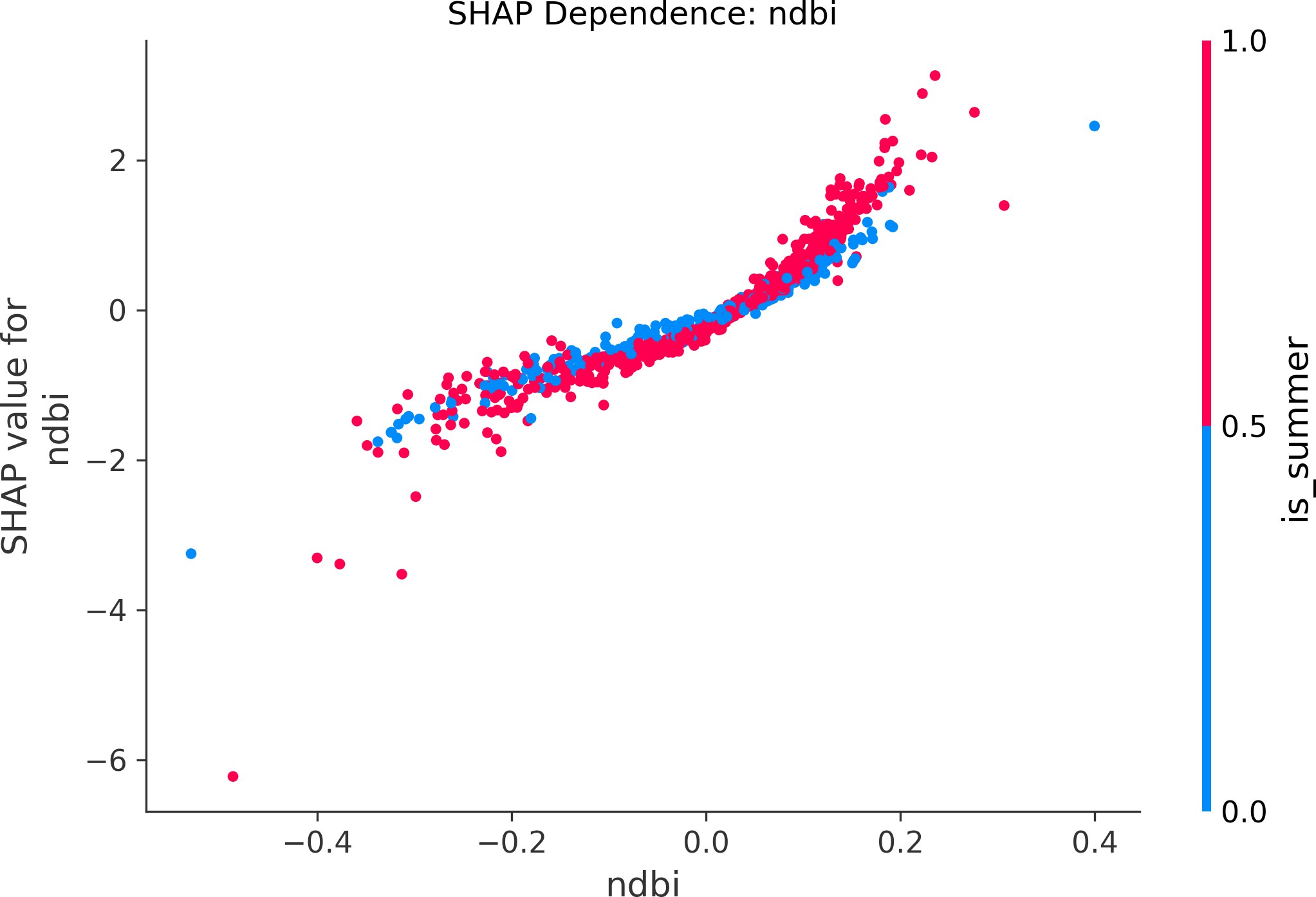
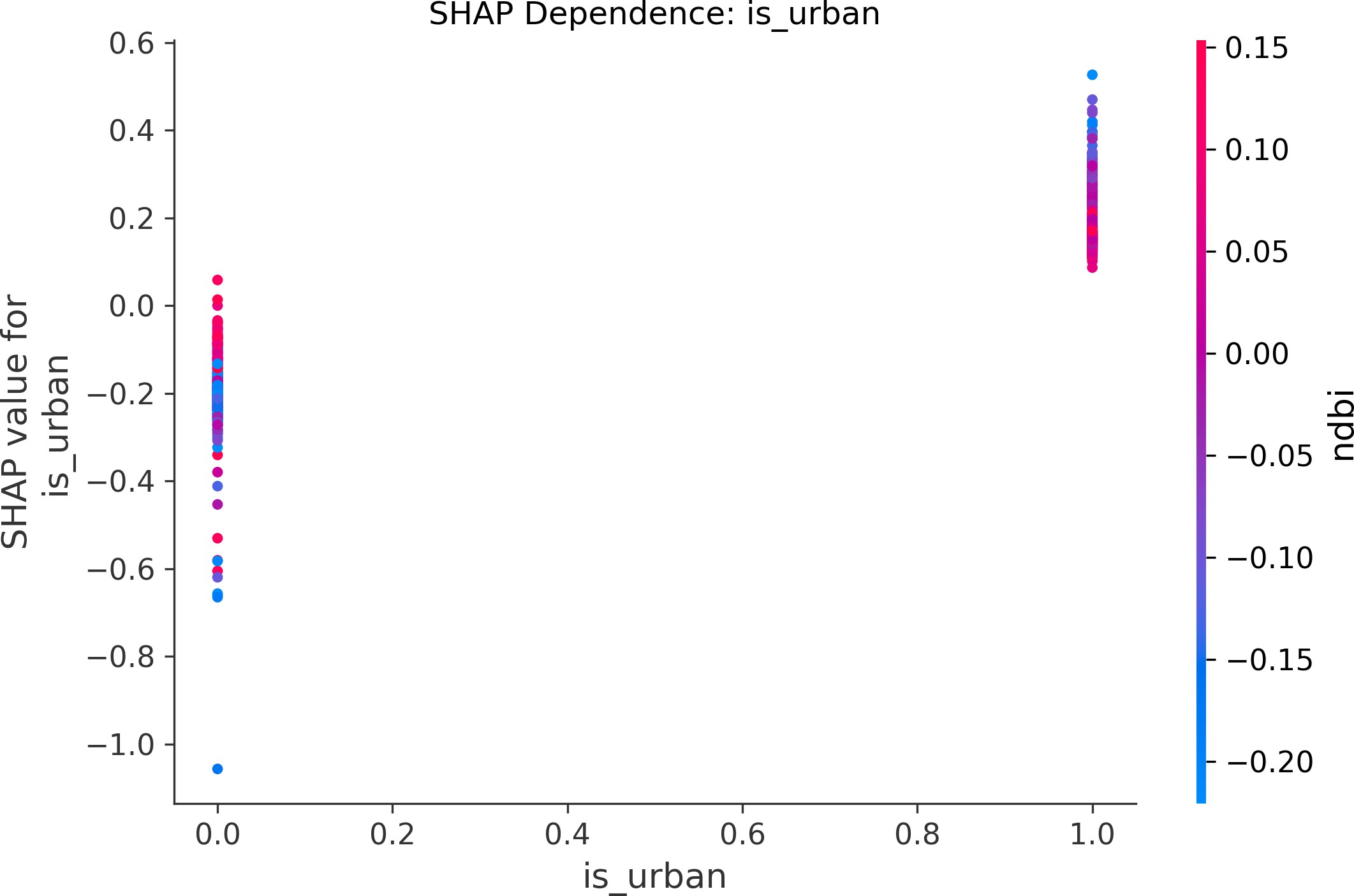
Expected physical behavior appears in the SHAP analysis: NDVI contributes a cooling tendency, NDBI contributes a warming tendency, and seasonality is highly influential because summer and winter differ strongly in surface temperature.

SHAP feature importance bar chart. — Fig. 4. Global SHAP importance ranking.

SHAP beeswarm plot showing signed feature contributions. — Fig. 5. Signed SHAP contribution distribution.

SHAP dependence plot for NDVI. — Fig. 6. Increasing NDVI tends to reduce predicted temperature.

SHAP dependence plot for NDBI. — Fig. 7. Higher NDBI increases positive SHAP contribution.

SHAP dependence plot for the binary urban indicator. — Fig. 8. Urban-class samples have a positive SHAP shift.

For a local explanation, a prediction can be expressed as a baseline plus the sum of feature contributions:

T_pred(x) = basevalue + shap₁(x) + ... + shap_d(x)

Publication Gates and Reproducibility

The reported run includes pass/fail publication gates, drift envelope checks, and checksum records. These are used to make the manuscript traceable back to fixed artifacts rather than a loose sequence of notebooks.

Table 3. Gate and drift consistency results.
Check	Result	Status
Objective scorecard	5/5 (100%)	PASS
NDVI physical check	corr(NDVI,LST) = -0.558	PASS
NDBI physical check	corr(NDBI,LST) = 0.622	PASS
Seasonal UHI mean	1.65 K	PASS
Seasonal UHI range	1.31-2.29 K	PASS
Published envelope	within 0.6 to 2.6 K: 100%	PASS

Table 4. Observed risks and mitigation strategy.
Risk	Mitigation used in final run
Seasonal stack drift	Step-12 envelope check against published Bengaluru UHI range
Spatial leakage in training	Spatial block hold-out by tile identifiers
Masking artifacts and NaN regions	Feature gates and documented downstream consistency checks
Overclaiming external validation	MODIS used only for regional consistency interpretation
Reproducibility loss	Manifest plus SHA-256 checksum records for artifact integrity

Threats to Validity and Future Work

Three limitations are identified. First, valid pixel count is lower for some winter year-season combinations. Second, heuristic NDVI/NDBI visualization masks are used qualitatively rather than quantitatively. Third, Level-2 MODIS validation is interpreted as regional consistency rather than per-pixel supervisory ground truth.

Future work includes evaluating Random Forest and CNN-based benchmarks under the same spatial split and reproducibility framework, expanding the spatial and temporal extent, and strengthening controlled benchmark comparisons.

References

T. R. Oke, The energetic basis of the urban heat island, Quarterly Journal of the Royal Meteorological Society, 1982.
J. A. Voogt and T. R. Oke, Thermal remote sensing of urban climates, Remote Sensing of Environment, 2003.
Q. Weng, D. Lu, and J. Schubring, Estimation of land surface temperature-vegetation abundance relationship for urban heat island studies, Remote Sensing of Environment, 2004.
T. Chen and C. Guestrin, XGBoost: A scalable tree boosting system, KDD, 2016.
S. M. Lundberg and S.-I. Lee, A unified approach to interpreting model predictions, NIPS, 2017.
Y. Chen et al., Machine learning for urban heat island assessment from remote sensing data: A review, Remote Sensing, 2023.
W. Zhang et al., Landsat 8 LST retrieval and spatial-temporal migration capabilities based on random forest, Advances in Space Research, 2024.

Reproducible Spatiotemporal Urban Heat Island Modeling for Bengaluru Using Earth Observation and Machine Learning